How to create a quantum gate from a unitary matrix in Qiskit with code

Interested in learning how to program quantum computers? Then check out our Qiskit textbook Introduction to Quantum Computing with Qiskit.

Introduction

In this tutorial we will see how to construct a quantum logic gate from a unitary matrix.

In quantum computing unitary matrices are very important as they describe how quantum logic gates and circuits affect qubit states.

In Qiskit a quantum logic gate can be created from a unitary matrix using the Unitary class:

Unitary(data)

Where:

• data: This is the unitary matrix that will be encoded in to the logic gate

For example the Pauli X gate can be described using the following matrix:

Using the unitary class we can implement the Pauli-X gate like so:

circuit.unitary([[0,1],[1,0]],q[0])

Where [[0,1],[1,0]] is the matrix we wish to encode and q[0] is the target qubit.

Implementation

In this section we will go through the full implementation step by step. The matrix we will be implementing is the Pauli-X gate matrix.

Step 1: Import modules

from qiskit import QuantumRegister, ClassicalRegister
from qiskit import QuantumCircuit, execute
from qiskit.quantum_info.operators import Operator
from qiskit import Aer

Step 2: Initialise the Backend

The next step is to intialise the backend device. Since this is only a tutorial we will use the Aer unitary simulator:

backend = Aer.get_backend('aer_simulator')

Step 3: Create the circuit

The next step is to create the circuit. This is just a one qubit circuit that creates a Pauli-X gate using the unitary class. Then the qubit is measured.

q = QuantumRegister(1,'q')
c = ClassicalRegister(1,'c')

circuit = QuantumCircuit(q,c)

circuit.unitary([[0,1],[1,0]],q[0])
circuit.measure(q,c)

Step 4: Execute the circuit and obtain the results

job = execute(circuit, backend, shots=8192)

counts = job.result().get_counts()

print(counts)

Code

from qiskit import QuantumRegister, ClassicalRegister
from qiskit import QuantumCircuit, execute
from qiskit.quantum_info.operators import Operator
from qiskit import Aer

backend = Aer.get_backend('aer_simulator')

q = QuantumRegister(1,'q')
c = ClassicalRegister(1,'c')

circuit = QuantumCircuit(q,c)

circuit.unitary([[0,1],[1,0]],q[0])
circuit.measure(q,c)

print(circuit)

job = execute(circuit, backend, shots=8192)

counts = job.result().get_counts()

print(counts)

Output

Output showing the qubit has flipped from |0〉to |1〉

Photonic Quantum Computing with Perceval

Introduction

Interested in learning how to program quantum computers? Then check out our Qiskit textbook Introduction to Quantum Computing with Qiskit.

This tutorial is the first tutorial in the series on Photonic Quantum Computing with the Perceval API from Quandela. In this tutorial we will look how to install Perceval and then how to implement a simple optical circuit that uses a beam splitter to put qubits in to superposition.

What is Perceval?

Perceval is an open source framework developed by Quandela that allows users to compose and simulate photonic circuits. It allows users to implement a number of optical components from Beam splitters which we will be using in this tutorial to Polarizers, Phase Shifters, and single photon sources.

For more on Perceval go to the website here: https://perceval.quandela.net/

Installing Perceval

The Perceval API can be installed easily from pip. Simple go in to your terminal and type in:

pip install perceval-quandela

Implementing a Beam Splitter

Now that we have installed Perceval we can now create our first photonic quantum computing circuit! In this tutorial we will start simply by creating a 2 mode optical circuit that implements a beam splitter.

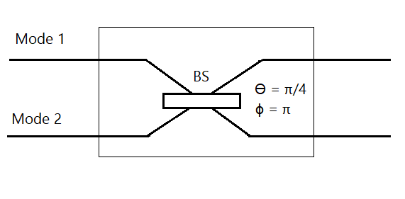
The beam splitter couples two spatial modes together. It can be defined using the following unitary matrix:

Where Θ corresponds to reflectivity of the beam splitter and Φ the relative phase between the two modes. Using matrix multiplication we can see how these parameters can affect the qubit states.

For our first example lets set the qubit state to |0〉and set the beam splitters parameters such that Θ = 0 and Φ = 0.

Remembering that the column vector associated with |0〉is:

Now we just need to multiply the matrix for the beam splitter with the column vector for |0〉:

Which has left the state unchanged.

If we instead set Θ = π/4 and Φ = 0:

Given that the the probability of a state occurring is the square of the state amplitude:

Probability of |0〉= 0.70710678118^2 = 0.5 or 50%

Probability of |1〉= 0.70710678118^2 = 0.5 or 50%

This shows that if we set Θ = π/4 and Φ = 0 we will have an equal superposition of states! This is also known as a 50:50 beam splitter.

Now that we have gone through how the beam splitter works we can now implement it using the Perceval API.

Step 1: Import the necessary modules

The first step in the code is to import the following modules:

• perceval: This is the main Perceval module

• perceval.lib.phys: The phys library contains all the components necessary to build the circuit

• sympy: A library used for symbolic mathematics

This is done with the following code:

import perceval as pcvl
import perceval.lib.phys as phys
import sympy as sp

Step 2: Build the Circuit

The next step is to build the circuit:

circuit = phys.Circuit(2)
circuit.add((0, 1), phys.BS(theta=sp.pi/4, phi_b=0))

phys.circuit(2) creates a circuit with 2 denoting the number of modes

circuit.add((0, 1), phys.BS(theta=sp.pi/4, phib=0)) adds a beam splitter to modes 0 and 1. Θ is set to π/4 and Φ (denoted as phi_b) is set to 0.

Step 3: Initialise the Backend

The next step is to pick the backend and pass the circuit to it:

simulator_backend = pcvl.BackendFactory().get_backend("Naive")
simulator = simulator_backend(circuit.U)

The first line picks the ‘Naive’ backend. There is a comparison table of the different backends in the documentation here: https://perceval.quandela.net/docs/backends.html

The second line passes the unitary matrix associated with the circuit to the backend.

Step 4: Use the Circuit Analyser to get the probability distribution

The final step is to use the circuit analyser to get the probability distribution of each output state. This is done with the following code:

ca = pcvl.CircuitAnalyser(simulator,[pcvl.BasicState([0, 1]), pcvl.BasicState([1, 0])])

pcvl.pdisplay(ca)

The first line passes the simulator and states to the Circuit analyser while the second line displays the probability distribution. The full code to implement the circuit as well as the output is below.

Code

import perceval as pcvl
import perceval.lib.phys as phys
import sympy as sp


circuit = phys.Circuit(2)
circuit.add((0, 1), phys.BS(theta=sp.pi/4, phi_b=0))


simulator_backend = pcvl.BackendFactory().get_backend("Naive")
simulator = simulator_backend(circuit.U)

ca = pcvl.CircuitAnalyser(simulator,[pcvl.BasicState([0, 1]), pcvl.BasicState([1, 0])])

pcvl.pdisplay(ca)

Output

Output showing the input and the corresponding output states. The 1/2 means there’s a 50% chance of the outcome happening. Therefore the states were in a superposition

Effects on T2 dephasing on IBM quantum computers

Introduction

Interested in learning how to program quantum computers? Then check out our Qiskit textbook Introduction to Quantum Computing with Qiskit.

In this tutorial we will explore the effects of T2 dephasing on IBM quantum computers in Qiskit.

What is T2 dephasing time?

Also known as T2 dephasing time this is where a qubits state dephases from either |+〉or |-〉to a mixture of phases such that the phase cannot be accurately predicted. For example if our initial state is |+〉then the state may decay to a mixture of |+〉and |-〉due to T2 dephasing.

The effects of T2 dephasing can be seen very easily with the following steps:

1. Put the qubit in to superposition using a Hadamard gate

2. Add a delay to the circuit

3. Bring the qubit out of superposition using another Hadamard gate

4. Measure the qubits state

The longer the delay the more measurements there will be for |1〉 due to dephasing.

Implementation

In Qiskit T2 dephasing can be observed very easily by with the following steps:

Step 1: Initialise the quantum and classical registers

The first step is to initialise the registers. Our circuit will consist of two registers. A quantum register that holds our qubit and a classical register that holds the bit used to hold the qubits state.

In Qiskit the registers can be initialized using the following code:

q = QuantumRegister(1,'q')
c = ClassicalRegister(1,'c')

Step 2: Create the circuit

The next step is to create the circuit. This consists of a Hadamard gate that is applied to the circuit followed by a delay of 283 microseconds. This is the average T2 dephasing time for the IBMQ Armonk device that is used in this tutorial. After this a second Hadamard gate is applied to bring the qubit out of superposition. Then finally the qubits state is measured.

circuit = QuantumCircuit(q,c)
circuit.h(q[0])
circuit.delay(283, unit="us") # Delay of 283 microseconds   
circuit.h(q[0])

circuit.measure(q[0],c[0]) #Measuring the qubit

Step 3: Transpile the circuit

The next step is to transpile the circuit. This is done so that the scheduling method can be set so that the delay will be implemented.

transpiled_circ = transpile(circuit, backend, scheduling_method='alap')  

Step 4: Execute the circuit on the backend device

Where nshots is the amount of times the circuit is ran and the backend is the ibmq_armonk device.

nShots = 8192
    
job = execute(transpiled_circ, backend, shots=nShots)
job_monitor(job)

Step 5: Get the results

The final step is to get the results back and print them!

counts = job.result().get_counts()

print("With delay: ",counts)

How to run the program

Copy and paste the code below in to a python file

1. Enter your API token in the IBMQ.enable_account('Insert API token here') part

2. Save and run

Note: To get an API key sign up to IBM Q Experience and get your token here: https://quantum-computing.ibm.com/account

Code

from qiskit import QuantumRegister, ClassicalRegister
from qiskit import QuantumCircuit, execute,IBMQ
from qiskit.tools.monitor import job_monitor
from qiskit import transpile
import numpy

pi = numpy.pi

IBMQ.enable_account('ENTER API KEY HERE')
provider = IBMQ.get_provider(hub='ibm-q')

backend = provider.get_backend('ibmq_armonk')

q = QuantumRegister(1,'q')
c = ClassicalRegister(1,'c')

def withoutDelay():
    circuit = QuantumCircuit(q,c)

    circuit.h(q[0])
    circuit.h(q[0])
    circuit.measure(q[0],c[0]) #Measuring the qubit

    nShots = 8192

    job = execute(circuit, backend, shots=nShots)
    job_monitor(job)

    counts = job.result().get_counts()

    print("No delay: ",counts)

def withDelay():  
    circuit = QuantumCircuit(q,c)
    circuit.h(q[0])
    circuit.delay(283, unit="us") # Delay of 200.79 microseconds   
    circuit.h(q[0])

    circuit.measure(q[0],c[0]) #Measuring the qubit

    transpiled_circ = transpile(circuit, backend, scheduling_method='alap')  

    nShots = 8192
    
    job = execute(transpiled_circ, backend, shots=nShots)
    job_monitor(job)

    counts = job.result().get_counts()

    print("With delay: ",counts)

withoutDelay()
withDelay()

Output

Output showing a significant number of counts for ‘1’ due to dephasing when there is a delay compared to with no delay.

Introduction to the U gate in Qiskit with Code

Interested in learning how to program quantum computers? Then check out our Qiskit textbook Introduction to Quantum Computing with Qiskit.

Introduction

In this tutorial we will explore the U gate and how to implement it in Qiskit on IBM Quantum Computers.

What is the U gate?

The U gate is a gate that does a rotation around the Bloch sphere with 3 Euler angles. The three angles used to perform the rotations are θ,λ, and φ.

The operation of the U can be described with the following matrix:

The U gate can replicate any other single qubit gate. For example to replicate the Pauli-X gate you would rotate θ by π, φ by π and λ by π/2 :

Where U(π, π, π/2 ) = U(θ, φ, λ)

As an example lets replicate a Pauli-X gate and set the qubit state to |1〉To see how the U gate operates on the qubit we multiply the column vector associated with |1〉by the U gate matrix.

This is correct as the resulting column vector is for |0〉This shows that the qubits state has flipped from |1〉to |0〉

If we wanted to use a U gate to create a Hadamard gate then the parameters would be set like so:

Let’s prove this by setting the qubit to |0〉 and then by multiplying the state vector by the U gate matrix with the parameters set as above:

Which has put the qubit in to superposition just as the Hadamard gate would!

Implementation

In Qiskit the U gate can be implemented very easily with the following line of code:

circuit.u(theta, phi, lam,q[0])

Where theta, phi, and lam are the 3 Euler angles and q[0] is the qubit that the U gate is applied to.

For example lets say we want to replicate a Pauli-X gate using the U gate. We will need to set theta and phi to π and lambda to π/2 like so:

circuit.u(pi, pi, pi/2,q[0])

How to run the program

Copy and paste the code below in to a python file

1. Enter your API token in the IBMQ.enable_account('Insert API token here') part

2. Save and run

Code

from qiskit import QuantumRegister, ClassicalRegister
from qiskit import QuantumCircuit, execute,IBMQ
from qiskit.tools.monitor import job_monitor
import numpy

pi = numpy.pi

IBMQ.enable_account('ENTER API KEY HERE')
provider = IBMQ.get_provider(hub='ibm-q')

backend = provider.get_backend('ibmq_qasm_simulator')

q = QuantumRegister(1,'q')
c = ClassicalRegister(1,'c')


circuit = QuantumCircuit(q,c)

circuit.u(pi,pi,pi/2,q[0]) # U3 Gate
circuit.measure(q,c) # Qubit Measurment

print(circuit)

job = execute(circuit, backend, shots=8192)
    
job_monitor(job)
counts = job.result().get_counts()

print(counts)

Output

Output showing the U gate has flipped the qubit from 0 to 1 much like an X gate

Introduction to the S gate in Qiskit with Code

Interested in learning how to program quantum computers? Then check out our Qiskit textbook Introduction to Quantum Computing with Qiskit.

Introduction

In this tutorial we will explore the S gate and how to implement on IBM quantum devices in Qiskit.

The S gate (otherwise known as the √Z gate) is a gate that performs a rotation of π/2 around the Z axis. It is represented by the following matrix:

Much like the Z gate if we initialise the qubit to |0〉and apply an S gate the qubits state will remain |0〉:

However if we first initialise the qubits state to |1〉:

Which has transformed the state from |1〉to i|1〉

It is important to note that since the S gate performs a rotation of π/2 if we apply two S gates we will get the equivalent of a Z gate:

Applying the first S gate:

Then the second S gate:

Which gives us −|1〉. This is correct as if we applied a Z gate to a qubit that is initialized to |1〉we would also get −|1〉

Since two S gates are equivalent to a Z gate we can flip a qubit from |0〉to |1〉by putting the qubit in to superposition, applying two S gates and then applying a closing Hadamard gate. To see how this works let’s go through step by step.

First initialise the qubit and apply a Hadamard gate:

Which has put the qubit in to superposition. Now if we apply the first S gate:

Now if we apply the second S gate:

and finally if we apply the closing Hadamard gate:

Which gives us |1〉as the final state! Note the full code below if for this example.

Impementation

The S gate can be implemented very easily in Qiskit using the following line of code:

circuit.s(q[0])

Where q[0] is the qubit we are applying the S gate to.

How to run the program

Copy and paste the code below in to a python file

1. Enter your API token in the IBMQ.enable_account('Insert API token here') part

2. Save and run

Code

from qiskit import QuantumRegister, ClassicalRegister
from qiskit import QuantumCircuit, execute,IBMQ
from qiskit.tools.monitor import job_monitor

IBMQ.enable_account('ENTER THE API KEY HERE')
provider = IBMQ.get_provider(hub='ibm-q')

backend = provider.get_backend('ibmq_qasm_simulator')

q = QuantumRegister(1,'q')
c = ClassicalRegister(1,'c')

circuit = QuantumCircuit(q,c)

circuit.h(q[0]) #Applying a Hadamard gate
circuit.s(q[0]) #Applying an S gate
circuit.s(q[0])
circuit.h(q[0]) #Applying another Hadamard gate to bring the qubit out of superposition
circuit.measure(q,c) #Measuring the qubit

print(circuit)

job = execute(circuit, backend, shots=8192)

job_monitor(job)
counts = job.result().get_counts()

print(counts)

Output

Output showing the circuit and that the qubit has flipped from 0 to 1